

Excelerating Analysis – Tips and Tricks to Analyze Data with Microsoft Excel
Incident response investigations don’t always involve standard host-based artifacts with fully developed parsing and analysis tools. At FireEye Mandiant, we frequently encounter incidents that involve a number of systems and solutions that utilize custom logging or artifact data. Determining what happened in an incident involves taking a dive into whatever type of data we are presented with, learning about it, and developing an efficient way to analyze the important evidence.
One of the most effective tools to perform this type of analysis is one that is in almost everyone’s toolkit: Microsoft Excel. In this article we will detail some tips and tricks with Excel to perform analysis when presented with any type of data.
Summarizing Verbose Artifacts
Tools such as FireEye Redline include handy timeline features to combine multiple artifact types into one concise timeline. When we use individual parsers or custom artifact formats, it may be tricky to view multiple types of data in the same view. Normalizing artifact data with Excel to a specific set of easy-to-use columns makes for a smooth combination of different artifact types.
Consider trying to review parsed file system, event log, and Registry data in the same view using the following data.
|
$SI Created |
$SI Modified |
File Name |
File Path |
File Size |
File MD5 |
File Attributes |
File Deleted |
|
2019-10-14 23:13:04 |
2019-10-14 23:33:45 |
Default.rdp |
C:Users |
485 |
c482e563df19a40 |
Archive |
FALSE |
|
Event Gen Time |
Event ID |
Event Message |
Event Category |
Event User |
Event System |
|
2019-10-14 23:13:06 |
4648 |
A logon was attempted using explicit credentials. Subject: |
Logon |
Administrator |
SourceSystem |
|
KeyModified |
Key Path |
KeyName |
ValueName |
ValueText |
Type |
|
2019-10-14 23:33:46 |
HKEY_USERSoftwareMicrosoftTerminal Server ClientServers |
DestinationServer |
UsernameHInt |
VictimUser |
REG_SZ |
Since these raw artifact data sets have different column headings and data types, they would be difficult to review in one timeline. If we format the data using Excel string concatenation, we can make the data easy to combine into a single timeline view. To format the data, we can use the “&” operation with a function to join information we may need into a “Summary” field.
An example command to join the relevant file system data delimited by ampersands could be “=D2 & ” | ” & C2 & ” | ” & E2 & ” | ” & F2 & ” | ” & G2 & ” | ” & H2”. Combining this format function with a “Timestamp” and “Timestamp Type” column will complete everything we need for streamlined analysis.
|
Timestamp |
Timestamp Type |
Event |
|
2019-10-14 23:13:04 |
$SI Created |
C:UsersattackerDocuments | Default.rdp | 485 | c482e563df19a401941c99888ac2f525 | Archive | FALSE |
|
2019-10-14 23:13:06 |
Event Gen Time |
4648 | A logon was attempted using explicit credentials. Subject: |
|
2019-10-14 23:33:45 |
$SI Modified |
C:UsersattackerDocuments | Default.rdp | 485 | c482e563df19a401941c99888ac2f525 | Archive | FALSE |
|
2019-10-14 23:33:46 |
KeyModified |
HKEY_USERSoftwareMicrosoftTerminal Server ClientServers | DestinationServer | UsernameHInt | VictimUser |
After sorting by timestamp, we can see evidence of the “DomainCorpAdministrator” account connecting from “SourceSystem” to “DestinationServer” with the “DomainCorpVictimUser” account via RDP across three artifact types.
Time Zone Conversions
One of the most critical elements of incident response and forensic analysis is timelining. Temporal analysis will often turn up new evidence by identifying events that precede or follow an event of interest. Equally critical is producing an accurate timeline for reporting. Timestamps and time zones can be frustrating, and things can get confusing when the systems being analyzed span various time zones. Mandiant tracks all timestamps in Coordinated Universal Time (UTC) format in its investigations to eliminate any confusion of both time zones and time adjustments such as daylight savings and regional summer seasons.
Of course, various sources of evidence do not always log time the same way. Some may be local time, some may be UTC, and as mentioned, data from sources in various geographical locations complicates things further. When compiling timelines, it is important to first know whether the evidence source is logged in UTC or local time. If it is logged in local time, we need to confirm which local time zone the evidence source is from. Then we can use the Excel TIME() formula to convert timestamps to UTC as needed.
This example scenario is based on a real investigation where the target organization was compromised via phishing email, and employee direct deposit information was changed via an internal HR application. In this situation, we have three log sources: email receipt logs, application logins, and application web logs.
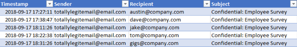
The email logs are recorded in UTC and contain the following information:
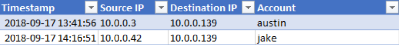
The application logins are recorded in Eastern Daylight Time (EDT) and contain the following:
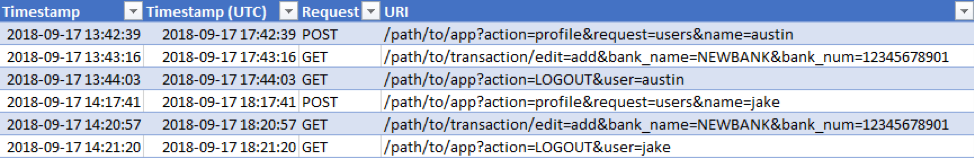
The application web logs are also recorded in Eastern Daylight Time (EDT) and contain the following:
To take this information and turn it into a master timeline, we can use the CONCAT function (an alternative to the ampersand concatenation used previously) to make a summary of the columns in one cell for each log source, such as this example formula for the email receipt logs:

This is where checking our time zones for each data source is critical. If we took the information as it is presented in the logs and assumed the timestamps were all in the same time zone and created a timeline of this information, it would look like this:
As it stands the previous screenshot, we have some login events to the HR application, which may look like normal activity for the employees. Then later in the day, they receive some suspicious emails. If this were hundreds of lines of log events, we would risk the login and web log events being overlooked as the time of activity precedes our suspected initial compromise vector by a few hours. If this were a timeline used for reporting, it would also be inaccurate.
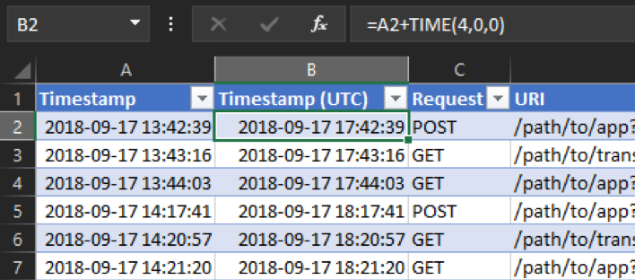
When we know which time zone our log sources are in, we can adjust the timestamps accordingly to reflect UTC. In this case, we confirmed through testing that the application logins and web logs are recorded in EDT, which is four hours behind UTC, or “UTC-4”. To change these to UTC time, we just need to add four hours to the time. The Excel TIME function makes this easy. We can just add a column to the existing tables, and in the first cell we type “=A2+TIME(4,0,0)”. Breaking this down:
- =A2
- Reference cell A2 (in this case our EDT timestamp). Note this is not an absolute reference, so we can use this formula for the rest of the rows.
- +TIME
- This tells Excel to take the value of the data in cell A2 as a “time” value type and add the following amount of time to it:
- (4,0,0)
- The TIME function in this instance requires three values, which are, from left to right: hours, minutes, seconds. In this example, we are adding 4 hours, 0 minutes, and 0 seconds.
Now we have a formula that takes the EDT timestamp and adds four hours to it to make it UTC. Then we can replicate this formula for the rest of the table. The end result looks like this:
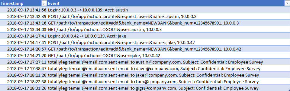
When we have all of our logs in the same time zone, we are ready to compile our master timeline. Taking the UTC timestamps and the summary events we made, our new, accurate timeline looks like this:
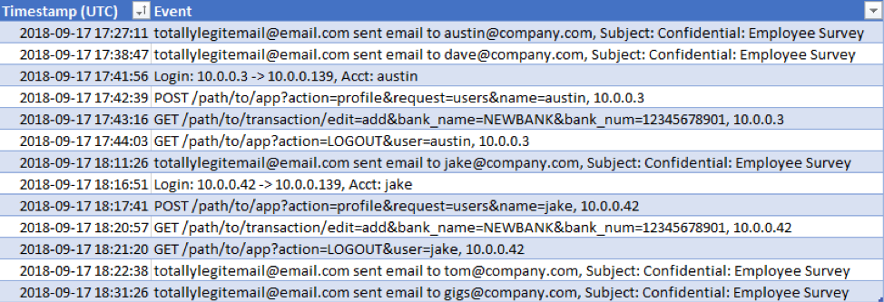
Now we can clearly see suspicious emails sent to (fictional) employees Austin and Dave. A few minutes later, Austin’s account logs into the HR application and adds a new bank account. After this, we see the same email sent to Jake. Soon after this, Jake’s account logs into the HR application and adds the same bank account information as Austin’s. Converting all our data sources to the same time zone with Excel allowed us to quickly link these events together and easily identify what the attacker did. Additionally, it provided us with more indicators, such as the known-bad bank account number to search for in the rest of the logs.
Pro Tip: Be sure to account for log data spanning over changes in UTC offset due to regional events such as daylight savings or summer seasons. For example, local time zone adjustments will need to change for logs in United States Eastern Time from Virginia, USA from +TIME(5,0,0) to +TIME(4,0,0) the first weekend in March every year and back from +TIME(4,0,0) to +TIME(5,0,0) the first weekend in November to account for daylight and standard shifts.
CountIf for Log Baselining
When reviewing logs that record authentication in the form of a user account and timestamp, we can use COUNTIF to establish simple baselines to identify those user accounts with inconsistent activity.
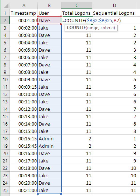
In the example of user logons that follows, we’ll use the formula “=COUNTIF($B$2:$B$25,B2)” to establish a historical baseline. Here is a breakdown of the parameters for this COUNTIF formula located in C2 in our example:
- COUNTIF
- This Excel formula counts how many times a value exists in a range of cells.
- $B$2:$B$25
- This is the entire range of all cells, B2 through B25, that we want to use as a range to search for a specific value. Note the use of “$” to ensure that the start and end of the range are an absolute reference and are not automatically updated by Excel if we copy this formula to other cells.
- B2
- This is the cell that contains the value we want to search for and count occurrences of in our range of $B$2:$B$25. Note that this parameter is not an absolute reference with a preceding “$”. This allows us to fill the formula down through all rows and ensure that we are counting the applicable user name.
To summarize, this formula will search the username column of all logon data and count how many times the user of each logon has logged on in total across all data points.
When most user accounts log on regularly, a compromised account being used to logon for the first time may clearly stand out when reviewing total log on counts. If we have a specific time frame in mind, it may be helpful to know which accounts first logged on during that time.
The COUNTIF formula can help track accounts through time to identify their first log on which can help identify rarely used credentials that were abused for a limited time frame.
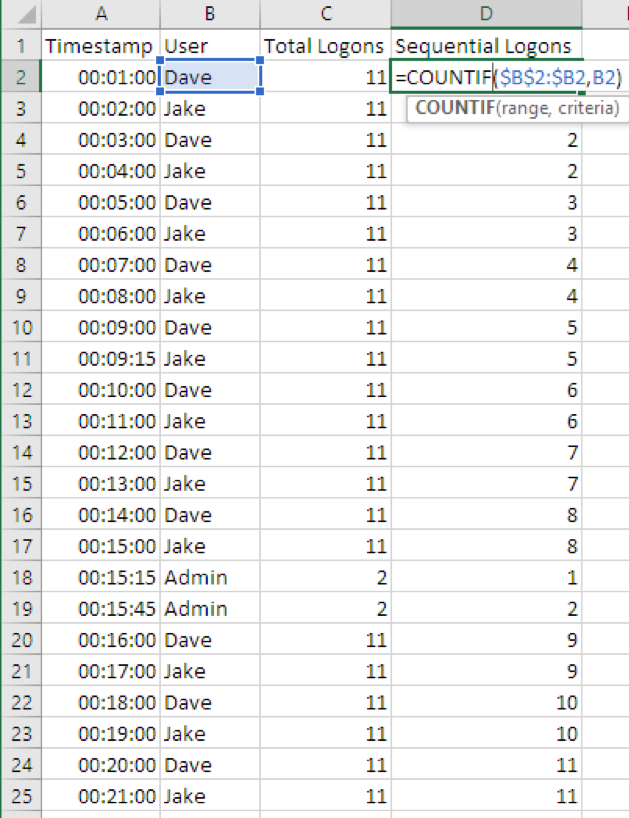
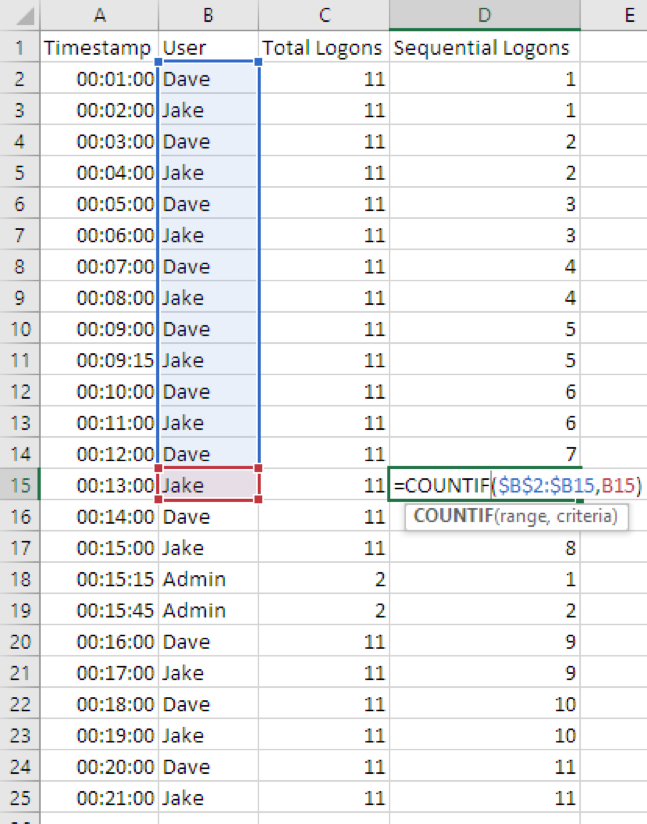
We’ll start with the formula “=COUNTIF($B$2:$B2,B2)” in cell D3. Here is a breakdown of the parameters for this COUNTIF formula. Note that the use of “$” for absolute referencing is slightly different for the range used, and that is an importance nuance:
- COUNTIF
- This Excel formula counts how many times a value exists in a range of cells.
- $B$2:$B2
- This is the range of cells, B2 through B2, that we want to start with. Since we want to increase our range as we go through the rows of the log data, the ending cell row number (2 in this example) is not made absolute. As we fill this formula down through the rest of our log data, it will automatically expand the range to include the current log record and all previous logs.
- B2
- This cell contains the value we want to search for and provides a count of occurrences found in our defined range. Note that this parameter B2 is not an absolute reference with a preceding “$”. This allows us to fill the formula down through all rows and ensure that we are counting the applicable user name.
To summarize, this formula will search the username column of all logon data before and including the current log and count how many times the user of each logon has logged on up to that point in time.
The following example illustrates how Excel automatically updated the range for D15 to $B$2:$B15 using the fill handle.
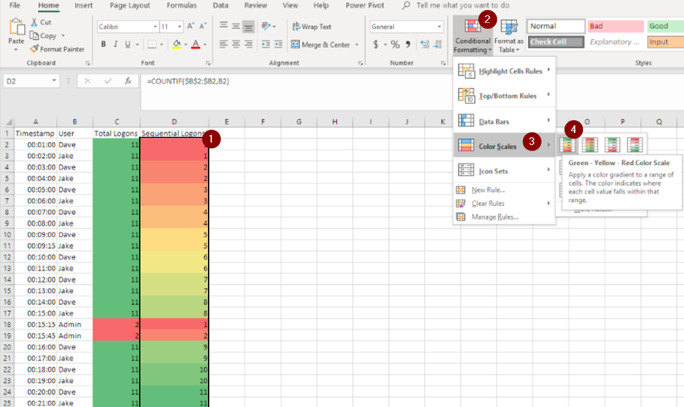
To help visualize a large data set, let’s add color scale conditional formatting to each row individually. To do so:
- Select only the cells we want to compare with the color scale (such as D2 to D25).
- On the Home menu, click the Conditional Formatting button in the Styles area.
- Click Color Scales.
- Click the type of color scale we would like to use.
The following examples set the lowest values to red and the highest values to green. We can see how:
- Users with lower authentication counts contrast against users with more authentications.
- The first authentication times of users stand out in red.
Whichever colors are used, be careful not to assume that one color, such as green, implies safety and another color, such as red, implies maliciousness.
Conclusion
The techniques described in this post are just a few ways to utilize Excel to perform analysis on arbitrary data. While these techniques may not leverage some of the more powerful features of Excel, as with any variety of skill set, mastering the fundamentals enables us to perform at a higher level. Employing fundamental Excel analysis techniques can empower an investigator to work through analysis of any presented data type as efficiently as possible.
This post was first first published on
‘s website by Jake Nicastro. You can view it by clicking here