Configuring a Windows Domain to Dynamically Analyze an Obfuscated Lateral Movement Tool

We recently encountered a large obfuscated malware sample that offered several interesting analysis challenges. It used virtualization that prevented us from producing a fully-deobfuscated memory dump for static analysis. Statically analyzing a large virtualized sample can take anywhere from several days to several weeks. Bypassing this time-consuming step presented an opportunity for collaboration between the FLARE reverse engineering team and the Mandiant consulting team which ultimately saved many hours of difficult reverse engineering.

We suspected the sample to be a lateral movement tool, so we needed an appropriate environment for dynamic analysis. Configuring the environment proved to be essential, and we want to empower other analysts who encounter samples that leverage a domain. Here we will explain the process of setting up a virtualized Windows domain to run the malware, as well as the analysis techniques we used to confirm some of the malware functionality.

Preliminary Analysis

When analyzing a new malware sample, we begin with basic static analysis, where we can often get an idea of what type of sample it is and what it’s capabilities might be. We can use this to inform the subsequent stages of the analysis process and focus on the relevant data. We begin with a Portable Executable analysis tool such as CFF Explorer. In this case, we found that the sample is quite large at 6.64 MB. This usually indicates that the sample includes statically linked libraries such as Boost or OpenSSL, which can make analysis difficult.

Additionally, we noticed that the import table includes eight dynamically linked DLLs with only one imported function each as shown in Figure 1. This is a common technique used by packers and obfuscators to import DLLs that can later be used for runtime linking, without exposing the actual APIs used by the malware.

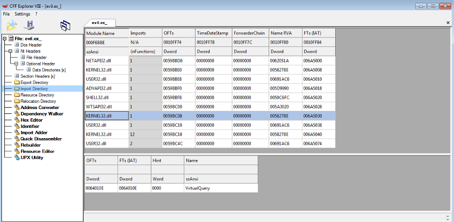
Figure 1: Suspicious imports

Our strings analysis confirmed our suspicion that the malware would be difficult to analyze statically. Because the file is so large, there were over 75,000 strings to consider. We used StringSifter to rank the strings according to relevance to malware analysis, but we did not identify anything useful. Figure 2 shows the most relevant strings according to StringSifter.

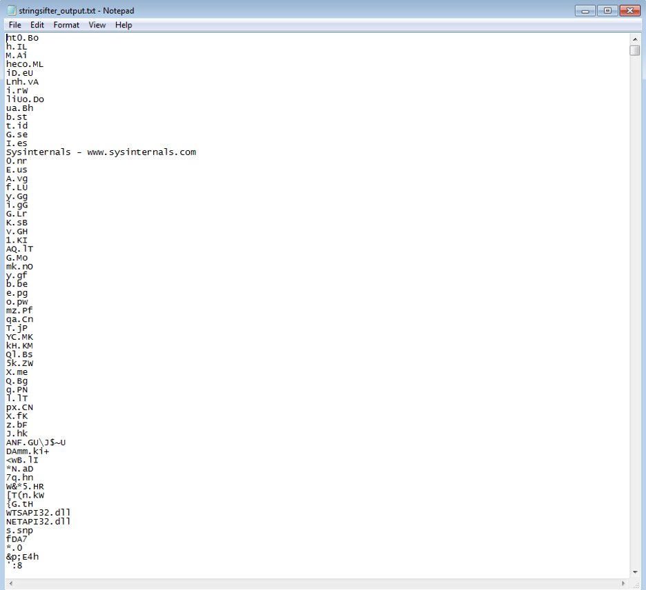
Figure 2: StringSifter output

When we encounter these types of obstacles, we can often turn to dynamic analysis to reveal the malware’s behavior. In this case, our basic dynamic analysis provided hope. Upon execution the sample printed a usage statement:

Usage: evil.exe [/P:str] [/S[:str]] [/B:str] [/F:str] [/C] [/L:str] [/H:str] [/T:int] [/E:int] [/R]    /P:str — path to payload file.    /S[:str] — share for reverse copy.    /B:str — path to file to load settings from.    /F:str — write log to specified file.    /C — write log to console.    /L:str — path to file with host list.    /H:str — host name to process.    /T:int — maximum number of concurrent threads.    /E:int — number of seconds to delay before payload deletion (set to 0 to avoid remove).    /R — remove payload from hosts (/P and /S will be ignored). If /S specifed without value, random name will be used. /L and /H can be combined and specified more than once. At least one must present. /B will be processed after all other flags and will override any specified values (if any). All parameters are case sensetive.

Figure 3: Usage statement

We attempted to unpack the sample by suspending the process and dumping the memory. This proved difficult as the malware exited almost instantly and deleted itself. We eventually managed to produce a partially-unpacked memory dump by using the commands in Figure 4.

sleep 2 && evil.exe /P:”C:WindowsSystem32calc.exe” /E:1000 /F:log.txt /H:some_host

Figure 4: Commands executed to run binary

We chose an arbitrary payload file and a large interval for payload deletion. We also provided a log filename and a hostname for payload execution. These parameters were designed to force a slower execution time so we could suspend the process before it terminated.

We used Process Dump to produce a memory snapshot after the two second delay. Unfortunately, virtualization still hindered static analysis and our sample remained mostly obfuscated, but we did manage to extract some strings which provided the breakthrough we needed.

Figure 5 shows some of the interesting strings we encountered that were not present in the original binary.

dumpedswaqp.exe psxexesvc schtasks.exe /create /tn “%s” /tr “%s” /s “%s” /sc onstart /ru system /f schtasks.exe /run /tn “%s” /s “%s” schtasks.exe /delete /tn “%s” /s “%s” /f ServicesActive Payload direct-copied Payload reverse-copied Payload removed Task created Task executed Task deleted SM opened Service created Service started Service stopped Service removed Total hosts: %d, Threads: %d SHARE_%c%c%c%c Share “%s” created, path “%s” Share “%s” removed Error at hooking API “%S” Dumping first %d bytes: DllRegisterServer DllInstall register install

Figure 5: Strings output from memory dump

Based on the analysis thus far, we suspected remote system access. However, we were unable to confirm our suspicions without providing an environment for lateral movement. To expedite analysis, we created a virtualized Windows domain.

This requires some configuration, so we have documented the process here to aid others when using this analysis technique.

Building a Test Environment

In the test environment, make sure to have clean Windows 10 and Windows Server 2016 (Desktop Experience) virtual machines installed. We recommend creating two Windows Server 2016 machines so the Domain Controller can be separated from the other test systems.

In VMware Virtual Network Editor on the host system, create a custom network with the following settings:

• Under VMNet Information, select the “Host-only” radio button.
• Ensure that “Connect a host virtual adapter” is disabled to prevent connection to the outside world.
• Ensure that the “Use local DHCP service” option is disabled if static IP addresses will be used.

This is demonstrated in Figure 6.

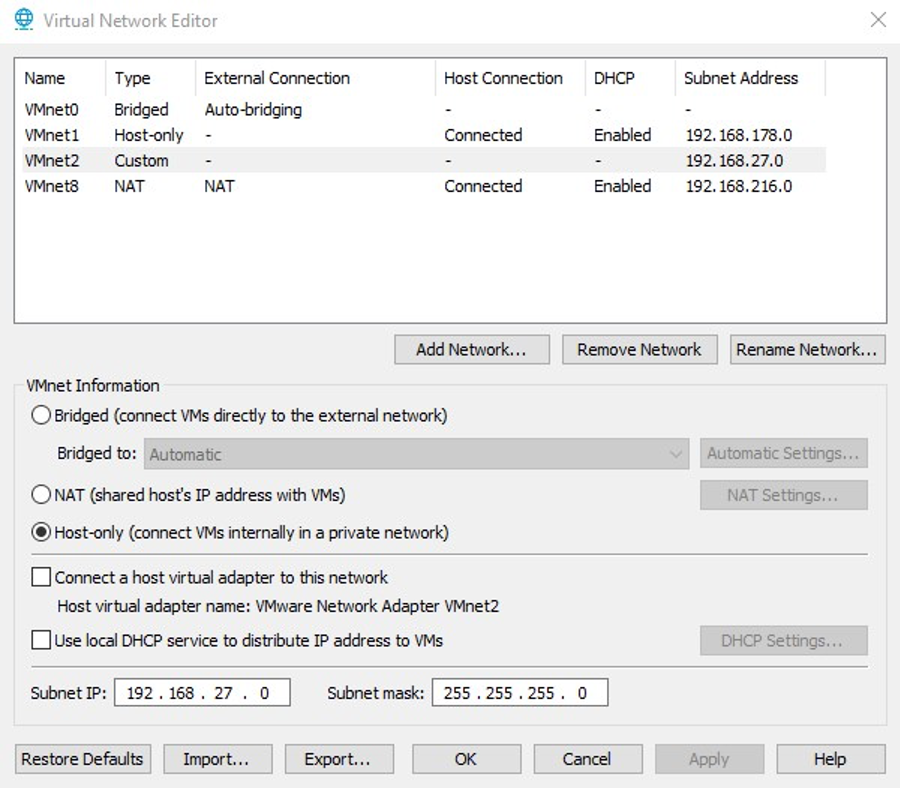
Figure 6: Virtual network adapter configuration

Then, configure the guests’ network adapters to connect to this network.

• Configure hostnames and static IP addresses for the virtual machines.
• Choose the domain controller IP as the default gateway and DNS server for all guests. 

We used the system configurations shown in Figure 7.

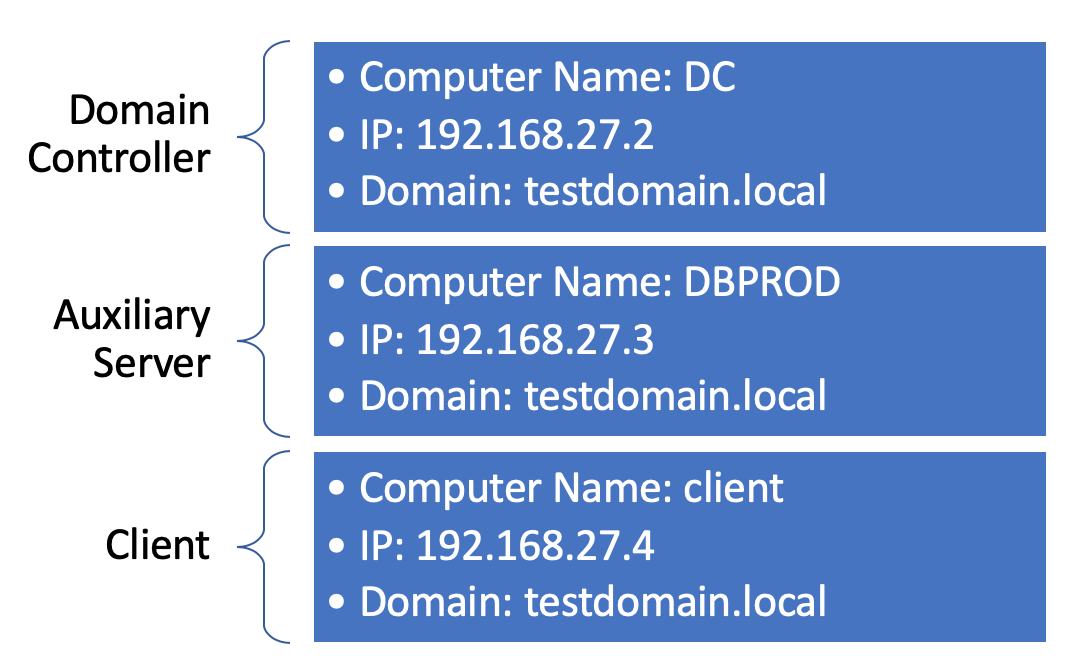
Figure 7: Example system configurations

Once everything is configured, begin by installing Active Directory Domain Services and DNS Server roles onto the designated domain controller server. This can be done by selecting the options shown in Figure 8 via the Windows Server Manager application. The default settings can be used throughout the dialog as roles are added.

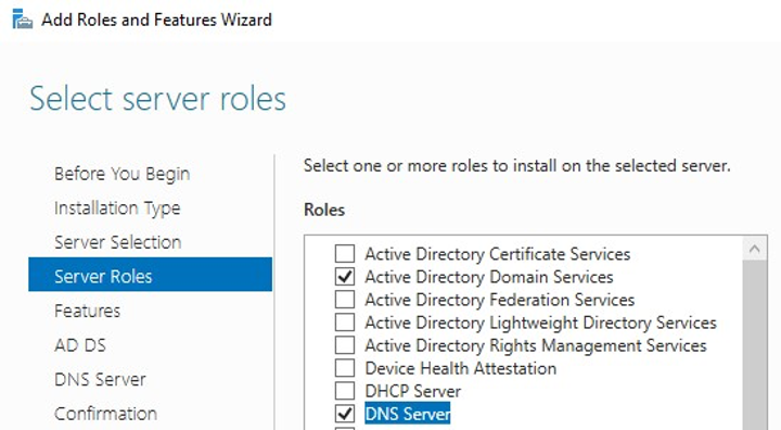
Figure 8: Roles needed on domain controller

Once the roles are installed, run the promotion operation as demonstrated in Figure 9. The promotion option is accessible through the notifications menu (flag icon) once the Active Directory Domain Services role is added to the server. Add a new forest with a fully qualified root domain name such as testdomain.local. Other options may be left as default. Once the promotion process is complete, reboot the system.

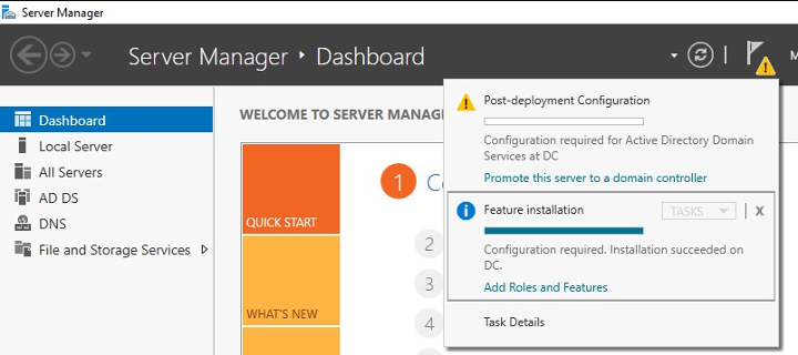
Figure 9: Promoting system to domain controller in Server Manager

Once the domain controller is promoted, create a test user account via Active Directory Users and Computers on the domain controller. An example is shown in Figure 10.

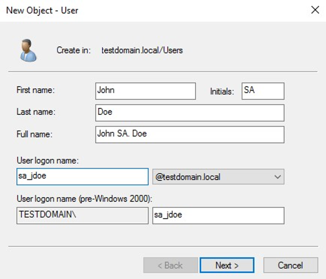
Figure 10: Test user account

Once the test account is created, proceed to join the other systems on the virtual network to the domain. This can be done through Advanced System Settings as shown in Figure 11. Use the test account credentials to join the system to the domain.

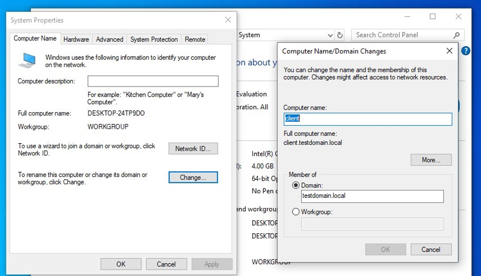
Figure 11: Configure the domain name for each guest

Once all systems are joined to the domain, verify that each system can ping the other systems. We recommend disabling the Windows Firewall in the test environment to ensure that each system can access all available services of another system in the test environment.

Give the test account administrative rights on all test systems. This can be done by modifying the local administrator group on each system manually with the command shown in Figure 12 or automated through a Group Policy Object (GPO).

net localgroup administrators sa_jdoe /ADD

Figure 12: Command to add user to local administrators group

Dynamic Analysis on the Domain

At this point, we were ready to begin our dynamic analysis. We prepared our test environment by installing and launching Wireshark and Process Monitor. We took snapshots of all three guests and ran the malware in the context of the test domain account on the client as shown in Figure 13.

evil.exe /P:”C:WindowsSystem32calc.exe” /L:hostnames.txt /F:log.txt /S /C

Figure 13: Command used to run the malware

We populated the hostnames.txt file with the following line-delimited hostnames as demonstrated in Figure 14.

DBPROD.testdomain.local client.testdomain.local DC.testdomain.local

Figure 14: File contents of hostnames.txt

Packet Capture Analysis

Upon analyzing the traffic in the packet capture, we identified SMB connections to each system in the host list. Before the SMB handshake completed, Kerberos tickets were requested. A ticket granting ticket (TGT) was requested for the user, and service tickets were requested for each server as seen in Figure 15. To learn more about the Kerberos authentication protocol, please see our recent blog post that introduces the protocol along with a new Mandiant Red Team tool.

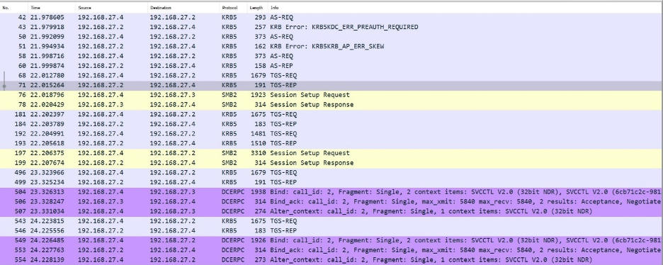
Figure 15: Kerberos authentication process

The malware accessed the C$ share over SMB and wrote the file C:Windowsswaqp.exe. It then used RPC to launch SVCCTL, which is used to register and launch services. SVCCTL created the swaqpd service. The service was used to execute the payload and then was subsequently deleted. Finally, the file was deleted, and no additional activity was observed. The traffic is shown in Figure 16.

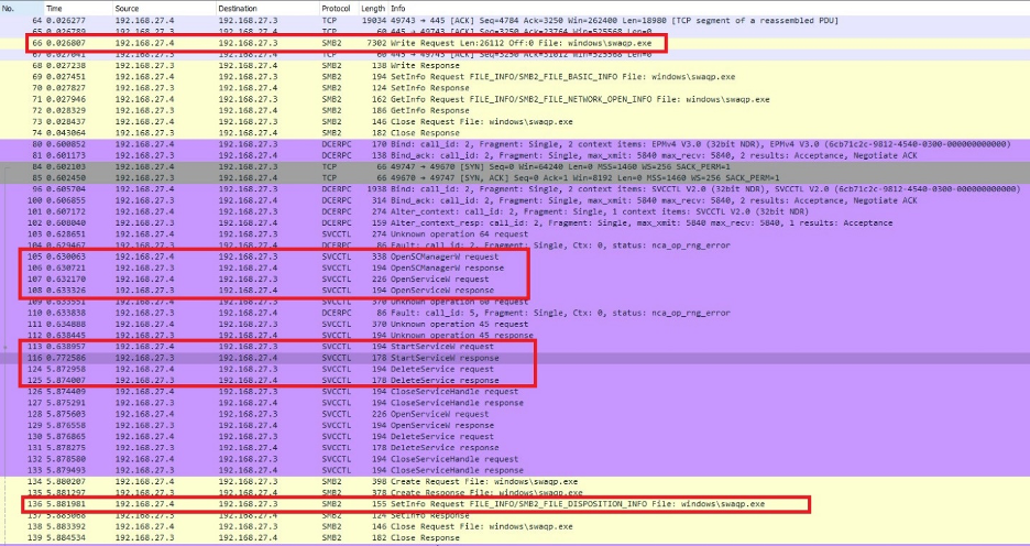
Figure 16: Malware behavior observed in packet capture

Our analysis of the malware behavior with Process Monitor confirmed this observation. We then proceeded to run the malware with different command line options and environments. Combined with our static analysis, we were able to determine with confidence the malware capabilities, which include copying a payload to a remote host, installing and running a service, and deleting the evidence afterward.

Conclusion

Static analysis of a large, obfuscated sample can take dozens of hours. Dynamic analysis can provide an alternate solution, but it requires the analyst to predict and simulate a proper execution environment. In this case we were able to combine our basic analysis fundamentals with a virtualized Windows domain to get the job done. We leveraged the diverse skills available to FireEye by combining FLARE reverse engineering expertise with Mandiant consulting and Red Team experience. This combination reduced analysis time to several hours. We supported an active incident response investigation by quickly extracting the necessary indicators from the compromised host. We hope that sharing this experience can assist others in building their own environment for lateral movement analysis.

This post was first first published on

‘s website by Matthew Haigh. You can view it by clicking here