

Excelerating Analysis, Part 2 — X[LOOKUP] Gon’ Pivot To Ya
In December 2019, we published a blog post on augmenting
analysis using Microsoft Excel for various data sets for
incident response investigations. As we described, investigations
often include custom or proprietary log formats and miscellaneous,
non-traditional forensic artifacts. There are, of course, a variety of
ways to tackle this task, but Excel stands out as a reliable way to
analyze and transform a majority of data sets we encounter.
In our first post, we discussed summarizing verbose artifacts using
the CONCAT function, converting timestamps using the TIME function,
and using the COUNTIF function for log baselining. In this post, we
will cover two additional versatile features of Excel: LOOKUP
functions and PivotTables.
For this scenario, we will use a dataset of logon events for an
example Microsoft Office 365 (O365) instance to demonstrate how an
analyst can enrich information in the dataset. Then we will
demonstrate some examples of how to use PivotTables to summarize
information and highlight anomalies in the data quickly.
Our data contains the following columns:
- Description – Event description
- User – User’s
name - User Principle Name – email address
- App – such
as Office 365, Sharepoint, etc. - Location – Country
- Date
- IP address
- User agent (simplified)
- Organization – associated with IP address (as identified by
O365)
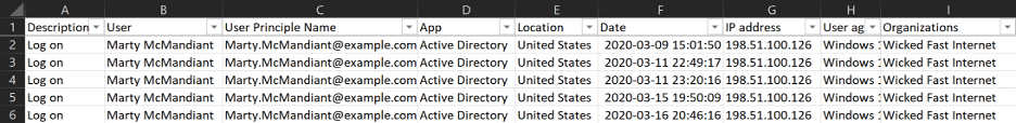
Figure 1: O365 data set
LOOKUP for Data Enrichment
It may be useful to add more information to the data that could help
us in analysis that isn’t provided by the original log source. A step
FireEye Mandiant often performs during investigations is to take all
unique IP addresses and query threat intelligence sources for each IP
address for reputation, WHOIS information, connections to known threat
actor activity, etc. This grants more information about each IP
address that we can take into consideration in our analysis.
While FireEye Mandiant is privy to historical engagement data and Mandiant
Threat Intelligence, if security teams or organizations do not
have access to commercial threat intelligence feeds, there are
numerous open source intelligence services that can be leveraged.
We can also use IP address geolocation services to obtain latitude
and longitude related to each source IP address. This information may
be useful in identifying anomalous logons based on geographical location.
After taking all source IP addresses, running them against threat
intelligence feeds and geolocating them, we have the following data
added to a second sheet called “IP Address Intel” in our Excel document:
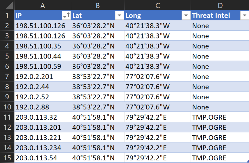
Figure 2: IP address enrichment
We can already see before we even dive into the logs themselves that
we have suspicious activity: The five IP addresses in the
203.0.113.0/24 range in our data are known to be associated with
activity connected to a fictional threat actor tracked as TMP.OGRE.
To enrich our original dataset, we will add three columns to our
data to integrate the supplementary information: “Latitude,”
“Longitude,” and “Threat Intel” (Figure 3). We can use the VLOOKUP or
XLOOKUP functions to quickly retrieve the supplementary data and
integrate it into our main O365 log sheet.
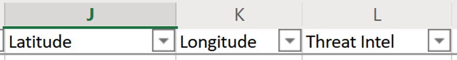
Figure 3: Enrichment columns
VLOOKUP
The traditional way to look up particular data in another array is
by using the VLOOKUP
function. We will use the following formula to reference the
“Latitude” values for a given IP address:
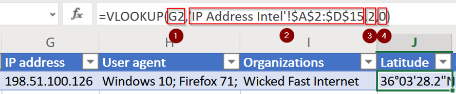
Figure 4: VLOOKUP formula for Latitude
There are four parts to this formula:
- Value to look up:
- This dictates what cell value we are
going to look up more information for. In this case, it is cell
G2, which is the IP address.
- This dictates what cell value we are
- Table
array:- This defines the entire array in which we will look
up our value and return data from. The first column in the array
must contain the value being looked up. In the aforementioned
example, we are searching in ‘IP Address Intel’!$A$2:$D:$15. In
other words, we are looking in the other sheet in this workbook
we created earlier titled “IP Address Intel”, then in that
sheet, search in the cell range of A2 to D15.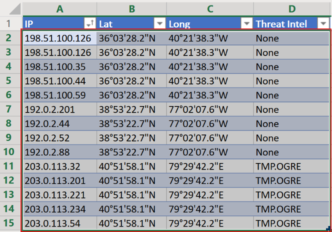 Figure 5: VLOOKUP table
array
Note the use of the “$” to ensure these are absolute
references and will not be updated by Excel if we copy this
formula to other cells.
- This defines the entire array in which we will look
- Column index
number:- This identifies the column number from which to
return data. The first column is considered column 1. We want to
return the “Latitude” value for the given IP address, so in the
aforementioned example, we tell Excel to return data from column
2.
- This identifies the column number from which to
- Range lookup (match type)
- This
part of the formula tells Excel what type of matching to perform
on the value being looked up. Excel defaults to “Approximate”
matching, which assumes the data is sorted and will match the
closest value. We want to perform “Exact” matching, so we put
“0” here (“FALSE” is also accepted).
- This
With the VLOOKUP function complete for the “Latitude” data, we can
use
the fill handle to update this field for the rest of the data set.
To get the values for the “Longitude” and “Threat Intel” columns, we
repeat the process by using a similar function and, adjusting the
column index number to reference the appropriate columns, then use the
fill handle to fill in the rest of the column in our O365 data sheet:
- For Longitude:
- =VLOOKUP(G2,’IP Address
Intel’!$A$2:$D$15,3,0)
- =VLOOKUP(G2,’IP Address
- For Threat
Intel:- =VLOOKUP(G2,’IP Address
Intel’!$A$2:$D$15,4,0)
- =VLOOKUP(G2,’IP Address
Bonus Option: XLOOKUP
The XLOOKUP
function in Excel is a more efficient way to reference the threat
intelligence data sheet. XLOOKUP is a newer function introduced to
Excel to replace the legacy VLOOKUP function and, at the time of
writing this post, is only available to “O365 subscribers in the
Monthly channel”, according to Microsoft. In this instance, we will
also leverage Excel’s dynamic
arrays and “spilling” to fill in this data more efficiently,
instead of making an XLOOKUP function for each column.
NOTE: To utilize dynamic arrays and spilling, the data we are
seeking to enrich cannot be in the form of a “Table” object. Instead,
we will apply filters to the top row of our O365 data set by selecting
the “Filter” option under “Sort & Filter” in the “Home” ribbon:
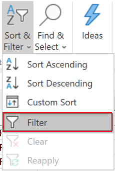
Figure 6: Filter option
To reference the threat intelligence data sheet using XLOOKUP, we
will use the following formula:
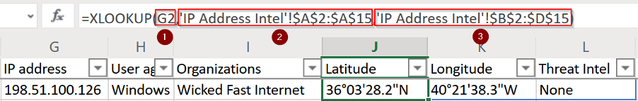
Figure 7: XLOOKUP function for enrichment
There are three parts to this XLOOKUP formula:
- Value to lookup:
- This dictates what cell value we are
going to look up more information for. In this case, it is cell
G2, which is the IP address.
- This dictates what cell value we are
- Array to look
in:- This will be the array of data in which Excel will
search for the value to look up. Excel does exact matching by
default for XLOOKUP. In the aforementioned example, we are
searching in ‘IP Address Intel’!$A$2:$A:$15. In other words, we
are looking in the other sheet in this workbook titled “IP
Address Intel”, then in that sheet, search in the cell range of
A2 to A15: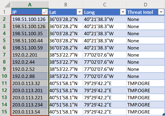 Figure 8: XLOOKUP array to look
in
Note the use of the “$” to ensure these are absolute
references and will not be updated by Excel if we copy this
formula to other cells.
- This will be the array of data in which Excel will
- Array of data to
return:- This part will be the array of data from which
Excel will return data. In this case, Excel will return the data
contained within the absolute range of B2 to D15 from the “IP
Address Intel” sheet for the value that was looked up. In the
aforementioned example formula, it will return the values in the
row for the IP address 198.51.100.126: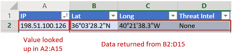 Figure 9: Data to be returned
from ‘IP Address Intel’ sheet
Because this is leveraging dynamic arrays and spilling,
all three cells of the returned data will populate, as seen in
Figure 4.
- This part will be the array of data from which
Now that our dataset is completely enriched by either using VLOOKUP
or XLOOKUP, we can start hunting for anomalous activity. As a quick
first step, since we know at least a handful of IP addresses are
potentially malicious, we can filter on the “Threat Intel” column for
all rows that match “TMP.OGRE” and reveal logons with source IP
addresses related to known threat actors. Now we have timeframes and
suspected compromised accounts to pivot off of for additional
hunting through other data.
PIVOT! PIVOT! PIVOT!
One of the most useful tools for highlighting anomalies by
summarizing data, performing frequency analysis and quickly obtaining
other statistics about a given dataset is Excel’s PivotTable function.
Location Anomalies
Let’s utilize a PivotTable to perform frequency analysis on the
location from which users logged in. This type of technique may
highlight activity where a user account logged in from a location
which is unusual for them.
To create a PivotTable for our data, we can select any cell in our
O365 data and select the entire range with Ctrl+A. Then, under the
“Insert” tab in the ribbon, select “PivotTable”:
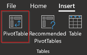
Figure 10: PivotTable selection
This will bring up a window, as seen in Figure 11, to confirm the
data for which we want to make a PivotTable (Step 1 in Figure 11).
Since we selected our O365 log data set with Ctrl+A, this should be
automatically populated. It will also ask where we want to put the
PivotTable (Step 2 in Figure 11). In this instance, we created another
sheet called “PivotTable 1” to place the PivotTable:
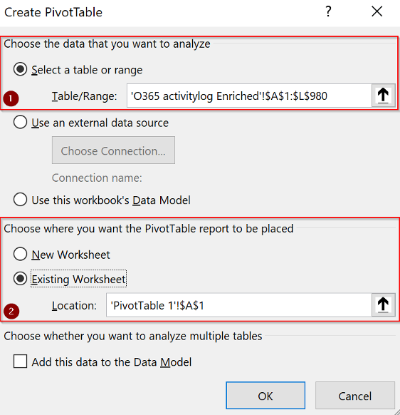
Figure 11: PivotTable creation
Now that the PivotTable is created, we must select how we want to
populate the PivotTable using our data. Remember, we are trying to
determine the locations from which all users logged in. We will want a
row for each user and a sub-row for each location the user has logged
in from. Let’s add a count of how many times they logged in from each
location as well. We will use the “Date” field to do this for this example:
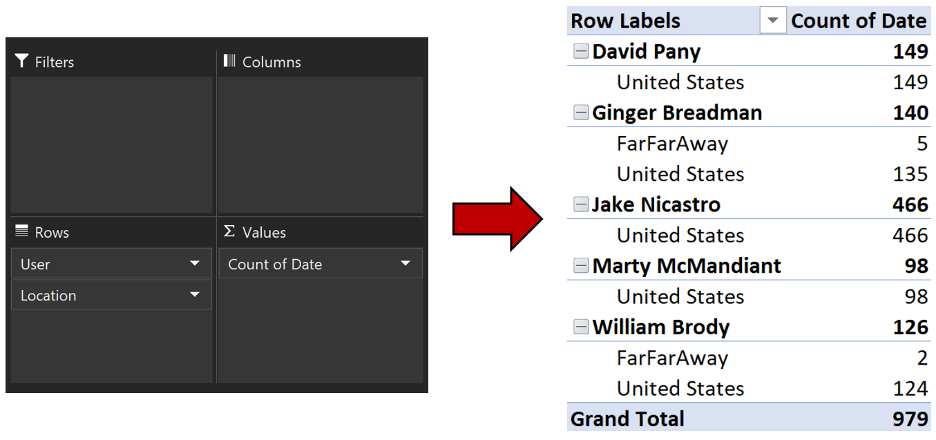
Figure 12: PivotTable field definitions
Examining this table, we can immediately see there are two users
with source location anomalies: Ginger Breadman and William Brody have
a small number of logons from “FarFarAway”, which is abnormal for
these users based on this data set.
We can add more data to this PivotTable to get a timeframe of this
suspicious activity by adding two more “Date” fields to the “Values”
area. Excel defaults to “Count” of whatever field we drop in this
area, but we will change this to the “Minimum” and “Maximum” values by
using the “Value Field Settings”, as seen in Figure 13.
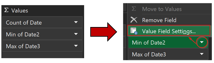
Figure 13: Adding min and max dates
Now we have a PivotTable that shows us anomalous locations for
logons, as well as the timeframe in which the logons occurred, so we
can hone our investigation. For this example, we also formatted all
cells with timestamp values to reflect the format FireEye Mandiant
typically uses during analysis by selecting all the appropriate cells,
right-clicking and choosing “Format Cells”, and using a “Custom”
format of “YYYY-MM-DD HH:MM:SS”.
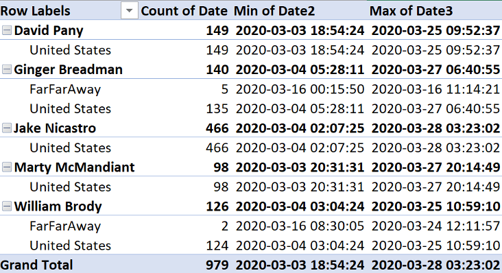
Figure 14: PivotTable with suspicious
locations and timeframe
IP Address Anomalies
Geolocation anomalies may not always be valuable. However, using a
similar configuration as the previous example, we can identify
suspicious source IP addresses. We will add “User Principle Name” and
“IP Address” fields as Rows, and “IP Address” as Values. Let’s also
add the “App” field to Columns. Our field settings and resulting table
are displayed in Figure 15:
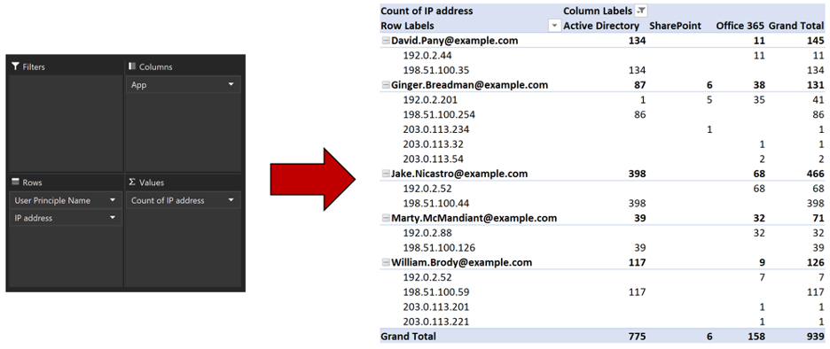
Figure 15: PivotTable with IP addresses
and apps
With just a few clicks, we have a summarized table indicating which
IP addresses each user logged in from, and which app they logged into.
We can quickly identify two users logged in from IP addresses in the
203.0.113.0/24 range six times, and which applications they logged
into from each of these IP addresses.
While these are just a couple use cases, there are many ways to
format and view evidence using PivotTables. We recommend trying
PivotTables on any data set being reviewed with Excel and
experimenting with the Rows, Columns, and Values parameters.
We also recommend adjusting the PivotTable
options, which can help reformat the table itself into a format
that might fit requirements.
Conclusion
These Excel functions are used frequently during investigations at
FireEye Mandiant and are considered important forensic analysis
techniques. The examples we give here are just a glimpse into the
utility of LOOKUP functions and PivotTables. LOOKUP functions can be
used to reference a multitude of data sources and can be applied in
other situations during investigations such as tracking remediation
and analysis efforts.
PivotTables may be used in a variety of ways as well, depending on
what data is available, and what sort of information is being analyzed
to identify suspicious activity. Employing these techniques, alongside
the ones we highlighted previously, on a consistent basis will go a
long way in “excelerating” forensic analysis skills and efficiency.